Introduction
The CHDU heat network model uses large multi-stage air source heat pumps (ASHPs) to provide most of the heat to the network. These heat pumps use electrically powered pumps to move heat from the air into the heat network. The efficiency of heat pumps at a single point in time is referred to as their coefficient of performance (COP) which is the ratio of the heat energy emitted to the electrical energy consumed. The instantaneous COP of an ASHP varies due to operating conditions such as the temperature of the air entering the unit, typically the outdoor ambient air temperature, and the temperatures of the incoming and outgoing coolant. The seasonal COP (SCOP) of the heat pump is calculated by dividing total heat energy generated within a calendar year by the total electrical energy consumed.
This article describes how the instantaneous COP of the ASHPs used in the CHDU techno-economic model (TEM) is calculated.
Air Temperature
The COP of an ASHP is sensitive to the ambient air temperature, hence an hourly air temperature profile is required to estimate an hourly COP profile. Since the purpose of the CHDU techno-economic model is to inform a nationwide site search, this air temperature profile must be able to account for the different air temperatures at different locations in the country.
Hourly air temperature profiles from the year 2023 were extracted from Renewables Ninja at different latitudes across mainland GB spanning from Southampton to Inverness. These profiles are presented in Figure 1.
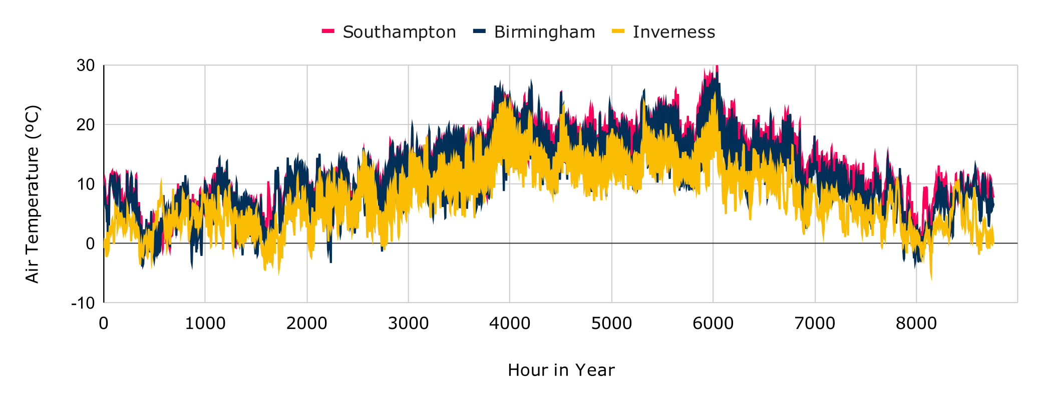
It is not feasible within the scope of the project to extract air temperature profiles at different locations across the country to accurately model the air temperature at specific heat network locations. Instead, the Birmingham air temperature profile has been adopted for use as the base air temperature profile in the CHDU techno-economic model. The air temperature profile at a specific location is generated by shifting the Birmingham air temperature profile by the difference between its average annual air temperature and the average annual air temperature of the target network site location. This means that the air temperature profile used to assess each site will have the same profile shape, but different hourly air temperature values.
To understand the implications of this approach, ASHP SCOP values were calculated using site specific air temperature profiles at different locations and the adjusted Birmingham air temperature profile. The results of the comparison are presented in Table 1.
| Location | SCOP – Site Specific Profile | SCOP – Adjusted Birmingham Profile | % difference |
| Inverness | 2.85 | 2.83 | 0.74% |
| Edinburgh | 2.90 | 2.88 | 0.77% |
| Glasgow | 2.90 | 2.88 | 0.87% |
| Carlisle | 2.90 | 2.88 | 0.66% |
| Leeds | 2.91 | 2.90 | 0.31% |
| Birmingham | 2.95 | 2.95 | 0.0% |
| Benson | 2.96 | 2.97 | -0.2% |
| Southampton | 3.01 | 3.00 | 0.17% |
The values presented in Table 1 suggest that there is not a significant difference in SCOP when using the Birmingham air temperature profile adjusted to match the mean air temperature of the site compared to using site specific profiles, with all locations having a difference within 1.5%. The comparison in Table 1 was reproduced for different demand profile shapes and produced comparable conclusions.
Sources of COP Values
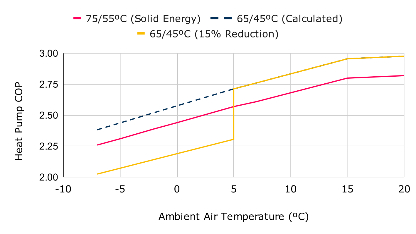
The ASHP manufacturer Solid Energy provided COP values for different ambient temperatures and a flow/return temperature of 75ºC/55ºC. These values were linearly scaled to the expected flow/return temperature of the CHDU heat networks of 65ºC/45ºC using relationships derived from ASHP COP data extracted from PyLESA.
The source and calculated COP values are presented in Figure 2.
How ASHP COP is Modelled
The Birmingham air temperature profile presented in Figure 1 is adjusted so that the mean temperature matches the target mean air temperature at a specific site (a model input). This is achieved by calculating the difference between the target mean air temperature and the mean air temperature of the Birmingham profile, then summing the difference with each hourly value in the Birmingham profile.
An hourly COP profile is then calculated by applying each hourly air temperature value to the 65ºC/45ºC COP relationship presented in Figure 2. This COP profile is used alongside the hourly heat demand profile to determine the hourly electrical demand of the ASHP.
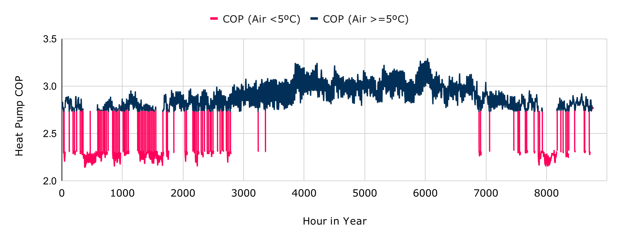
An example of the resulting hourly COP profile is presented in Figure 3. Note that the SCOP for the presented profile is 2.97.
References
HeatGeek, https://www.heatgeek.com/how-are-heat-pumps-over-100-efficient/
PyLESA: https://stax.strath.ac.uk/concern/theses/q811kk106
Solid Energy, https://www.solid-group.dk/en/solid-energy/
Banner Image Attribution:
Image sourced from commons.wikimedia.org and licensed under the Creative Commons Attribution-Share Alike 4.0 International license.